A gentle introduction to tensor networks

I have been actively nerd-sniping recruits to the cult of tensor networks. While this has been great, I keep promising greatness without backing that up. This post provides an introductory overview of the topic for the newly initiated. This post is aimed at interpretability researchers.

While the central concept behind tensor networks is not very difficult, the literature can be daunting. In contrast, this post is vibe-written, distilling the main ideas succinctly and (hopefully) clearly. Do not expect rigour (or even correctness).

This tutorial offers a range of references, along with some preliminary explanations and intuition, to help get started with a specific set of papers. The final goal is for this to become a self-contained booklet. However, apparently, distilling a deeply technical field into bite-sized concepts is challenging.

This tutorial contains four parts.

• What are tensor networks?
• Tensor networks generalise decompositions.
• Cool algorithms for tensor networks.
• Generalising ‘structure’ with tensor networks.

What are tensor networks?

Tensors are generalisations of matrices that describe complex interactions between an arbitrary number of sources, often referred to as modes. In contrast, matrices define linear relations between two modes, but tensors allow arbitrarily many. The drawback is that most tensors are intractable to store. Assuming sources are of equal dimensionality $n$, a matrix contains $n^2$ entries, but tensors require $n^s$ entries depending on the number of sources $s$.

Consequently, tensors are generally never instantiated but rather defined in a compact manner using tensor networks. Tensor networks are graphs where the edges are contractions, and the nodes are tensors. Notably, tensor networks can (and should!) be denoted diagrammatically, which is genuinely extremely helpful. These diagrams allow one to reason about complex structures in a visual manner (and doodle while in the shower).

Unfortunately, I don’t think a proper introductory resource exists yet. I have a self-written (but incomplete) source about tensor diagrams. The following are (seen as) the defaults to learn about tensor networks. There is also an interpretability specific introduction. Unfortunately, I think that article doesn’t put sufficient emphasis on structure and algorithms.

You’ll see a stark contrast between papers that use proper diagrammatic notation and others that use old-school Einstein notation. I find the latter impossible to comprehend, even with extensive experience.

Tensor networks generalise decompositions

Tensor networks describe structured tensors, which equates to some form of decomposition. Matrix decompositions typically consist of only two or three structured parts — hardly a “network”. But, as we will see, tensors can be meaningfully described by arbitrarily complex networks.

We focus on two reasonable and straightforward tensor decompositions which generalise across orders: the canonical polyadic decomposition (CPD) and the Tucker decomposition (TD).

The CPD is known under many names, such as Candecomp/Parafac decomposition or tensor rank decomposition. This will be a recurring theme throughout; try to ignore this unfortunate confusion.

In short, the CPD is a sum of rank-1 outer products, which resembles the singular value decomposition (SVD) but with an outer product of three vectors. The CPD splits an order $k$ tensor into $k$ matrices with an outer product operation in the middle. Interestingly, a SwiGLU is precisely a CPD if you remove the Swish non-linearity. It describes how two inputs interact towards an output, making it an interesting object of study.

It’s generally accepted that this is the most meaningful generalisation of rank to arbitrary tensors. Unfortunately, computing this is NP-hard in general, and there are almost no meaningful bounds to reason about this rank. However, it’s known tensor rank saturates at $\min_j(\prod^{k}_{i \neq j} n_i)$ (lowest product of all mode dimensions except one), just like matrix rank saturates at $\min(n, m)$ (where n and m are the dimensions, which is just a special case of the tensor formula).

This is quite useful because you can quantify how much ‘signal’ the tensor network is capturing instead of just populating the whole product space.

The TD comprises a down-projection for each mode, combined with a tensor ‘core’ that contains the higher-order interactions, albeit in a compressed format. See this seminal (albeit old) paper for more details/rigour.

• The CPD represents a sum of simple interactions-> simple computation but in high dimensions.
• The TD compresses its higher-order interactions-> complex computation but in lower dimensions.

You may wonder if there’s something in between, and the answer is yes! Let’s generalise a bit; there are two variables to this (this has a bunch of official names, so I’m going to use what makes the most sense to me).

• The factor dimension is 1 for a CPD and high for a TD. I refer to this as the complexity of interactions/computations.
• The factor amount is high for a CPD but 1 for a TD. This intuitively means the amount of ‘distinct’ interactions.

From this viewpoint, it could make sense to trade off the amount of factors for a higher dimension for each. For instance, what if you changed the CPD such that each factor is dimension 2. Or, put differently, a sum of small TDs. This topic has been previously studied and lies at a fascinating intersection of compressed sensing and tensor networks.

The trade-off is helpful because if the underlying computation requires interactions of rank 2, it will take many CPD ($2^k$, I think) factors to represent this. So, finding these ‘joint’ factors is a good way to compress the computation/interactions. The notion of structure in tensor networks its geometric interpretation is formalised in the last section. In short, any form of structure, either through manifolds, bottlenecks, or (communication) flow constraints, is describable by this.

Before that, though, I want to talk about really high-order tensor networks. While it becomes harder to reason about, it’s not uncommon to want to describe interactions between thousands of sources. Here, the TD completely fails, even for factor dimension 2. The CPD is probably still storable but requires way too many parameters.

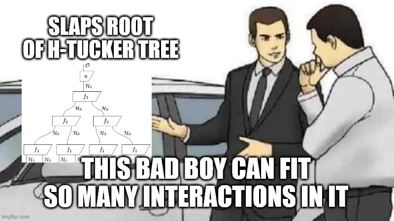
Enter hierarchical formats. Instead of defining a decomposition between all modes, we can introduce ‘hidden modes’. You can form a tensor tree where each decomposition only combines a few modes at a time in the form of a tree. This is known as an H(ierarchical)-Tucker decomposition. It’s also possible to use the CPD to describe intermediate interactions, although I have thus far failed to find a literature reference that studies this specific network class. In any case, this idea is often abstracted as “tree tensor networks”, where only a single path connects each mode. These are generally really nice to work with and have a variety of algorithms that work on them.

There exist specific decompositions (MERA/PEPS) that are not trees (they contain so-called loops) but still have many valuable properties. We do not discuss them here.

This marks the end of the tensor network whirlwind tour. These networks transparently encode interactions in a way that is easy to reason about while being extremely expressive.

Cool algorithms for tensor networks

Due to the generality of tensor networks, it’s possible to imagine arbitrarily complex algorithms. Luckily, many of them boil down to one core algorithm: diagonalisation. Diagonalisation extends the idea of matrix diagonalisation but operates on the connections of tensors. This enables one to assign a singular value to each dimension of the connection and potentially enables pruning really big parts of the network. This algorithm is also sometimes called canonicalisation because it reveals the most compressed and natural form of a tensor network.

In short, for each connection/edge/wire, we view both sides as two huge matrices, for which we compute the left and right singular values. Computing the singular values can be done extremely efficiently (for reasons that I don’t think I can explain in simple terms).

Even though this algorithm assumes a tree tensor network (such that both sides are disconnected), you can still perform this to get meaningful results in arbitrary networks.

I’ve only found one paper that is somewhat accessible on the topic. Then there are two papers, describing theory and algorithms which are insightful but basically impossible to understand by mere mortals. I tried writing a paper to distill these ideas, but it’s still a bit hard to grasp probably.

Generalising ‘structure’ with tensor networks

As said in a previous chapter, some tensor networks allow trading factor count for factor size. There, we provided an example of enhancing the CPD to have factors of size 2. Here, I explain how structure in the factor matrices influences the representable interactions.

One can rephrase the CPD of factor size 2 as a CPD of twice the hidden dimension, but where each factor matrix is constrained by a 2-block diagonal matrix (forcing rows/columns to be joint). This can be extended to sparsity; if the factor matrices admit a sparse decomposition, then this bounds the interactions into (small) groups of arbitrary size. See this website and this paper.

Tensor networks enable the definition of high-level interaction topologies, while structured matrices facilitate the definition of low-level interactions. Both are extremely meaningful in their own right and extremely useful to find any form of ‘structure’. Importantly, the interpretation of low-level structure is dependent on the higher-level structure and may lose meaning when complex non-linearities are introduced.

Especially sparsity is cool because, if sufficiently low ($<3$), it explains visualisable geometries. Since tensor networks can represent polynomials (interactions with oneself), suddenly, sparsity on a CPD implies low-degree polynomial manifolds like conic sections and circles!

Let me handwave my way through other forms of structure. For instance, ‘flow restriction’, where a given element can only interact with prior elements to enforce a specific order, is simply adding an upper or lower triangular matrix anywhere in the tensor network. Alternatively, matrices themselves can be represented as tensor networks, which constrain their representations in even more complicated (but potentially useful) ways, eg. Monarch matrices.

Conclusion

I hope this introduction has provided sufficient motivation behind tensor networks. The objects genuinely have a bunch of nice properties, not just in terms of expressiveness, but only on how to reason about them. Unfortunately, this knowledge is often hidden behind opaque theorems and inscrutable papers. My hope is to distill this knowledge toward pratical use-cases, especially in interpretability.